Spatial Holdouts and Feature Selection

Findings

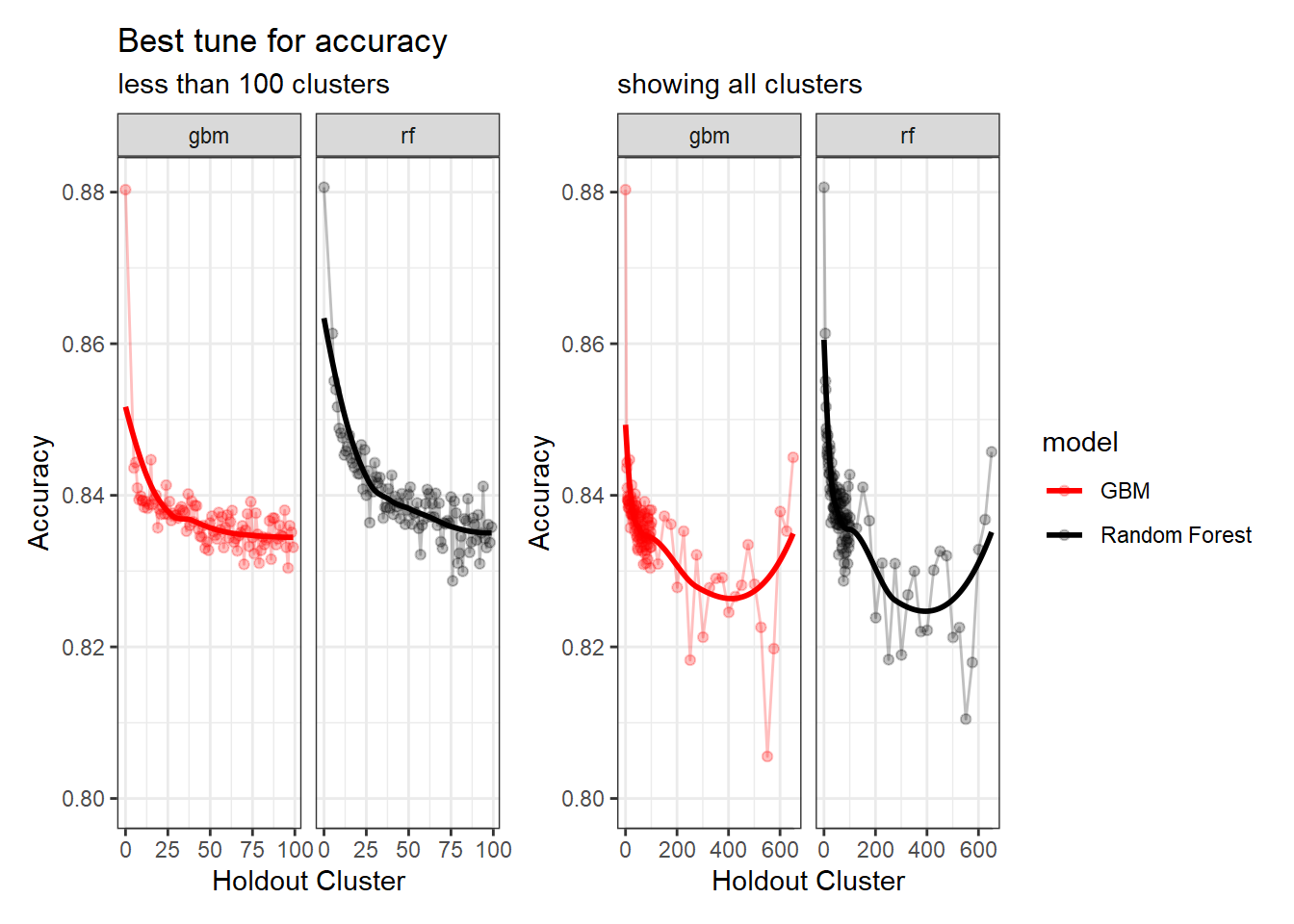
• Both model types (gbm and random forest) are very sensitive when using all variables and no spatial hold-outs; however, when increasing the hold out size (iid becomes more appropriate) we see that random forest takes some time before it stabilizes unlike gbm which is able to control for that effect early on.

• FFS variable selection at cluster holdout 10 was 9 variables while the new variable selection (unnamed) used only 5 variables at a cluster holdout of 10 while keeping the same accuracy; making the model more parsimonious.

• Difference between 10 and 100 holdout clusters is 0.001 in contrast to no holdouts (Random CV) and 10 the difference is 0.041.

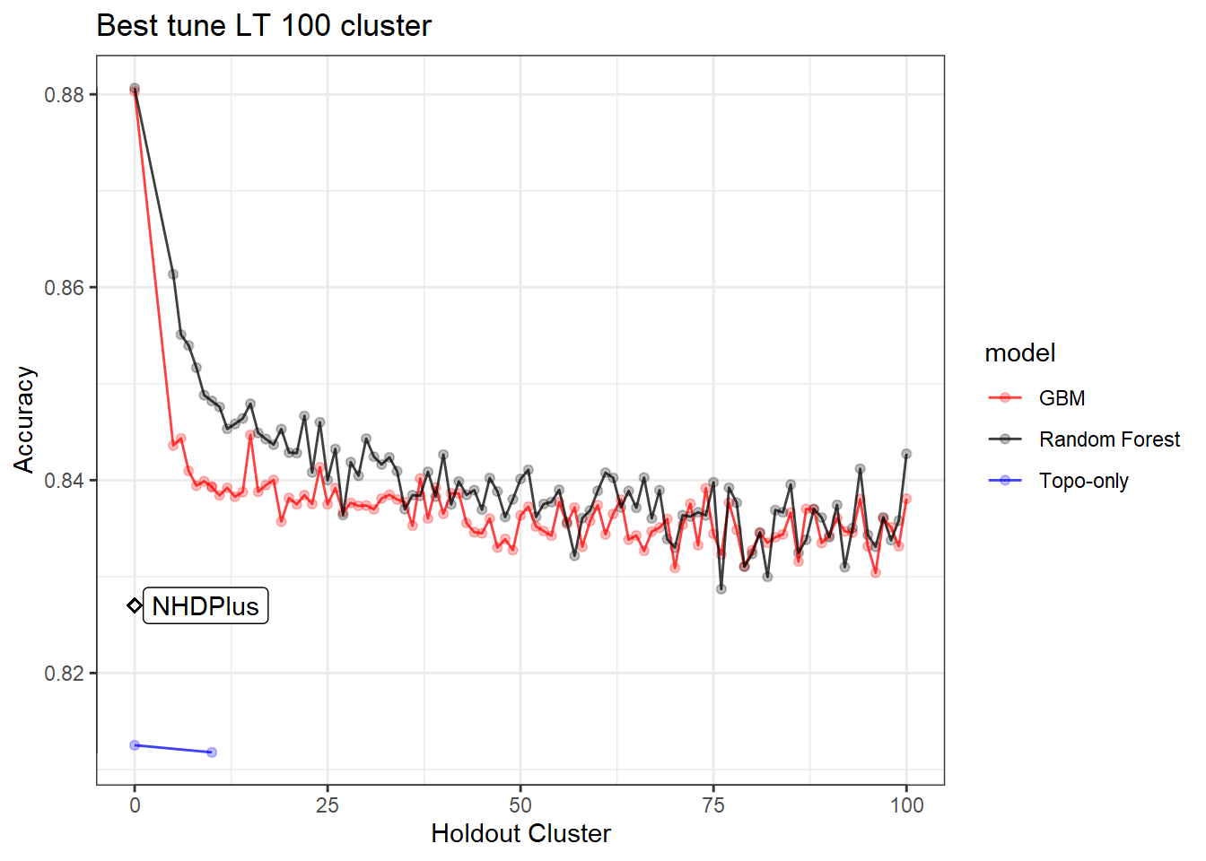
• Accuracy for GBM models: Random CV (0.88), Topoclimatic (0.839), Topography-only (0.812), NDHPlus (0.827).

Discussion

• There is a lot of interesting results not only in the stream prediction part but also in the model building process. How might this be improved or communicated so that others can use to their advantage?

• What are some possible limitations with this approach?

• The separation between the results are not so hard-hitting but do they shed some light into the advantages of using some remote sensing indices?

This is a exploration into picking a hold out set in the headwater stream prediction model. First read in the data and then clean it. This data includes 238 model runs (119 GBM/ 199 RF) at cluster holdouts of 5-100 and then a sequence of 101-651 by 25 along with 3 Random CV runs and two cluster of 10 tuned models for a total of 243 models. Below are plots of all these model runs and a loose interpretation in how the variables and holdout value were determined. Notice how steep the drop off is from Random CV (Holdout Cluster = 0) and 5 holdout.

Let’s look a little closer into the data where we have more model runs, e.g. less than 100.

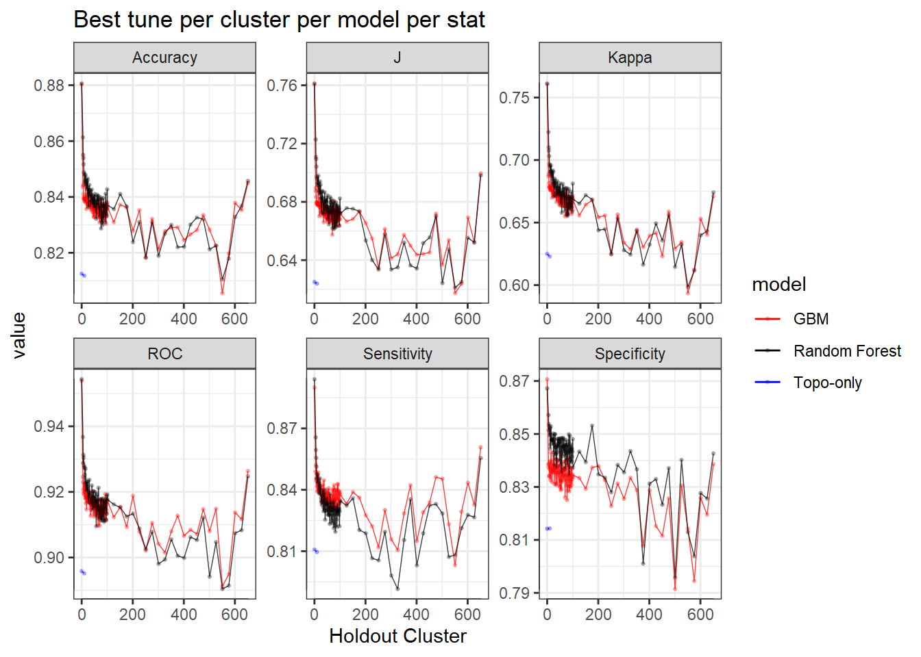
Now let’s look at other statistics, e.g. sensitivity, specificity, J, Kappa.

Now with standard deviation within each cluster.

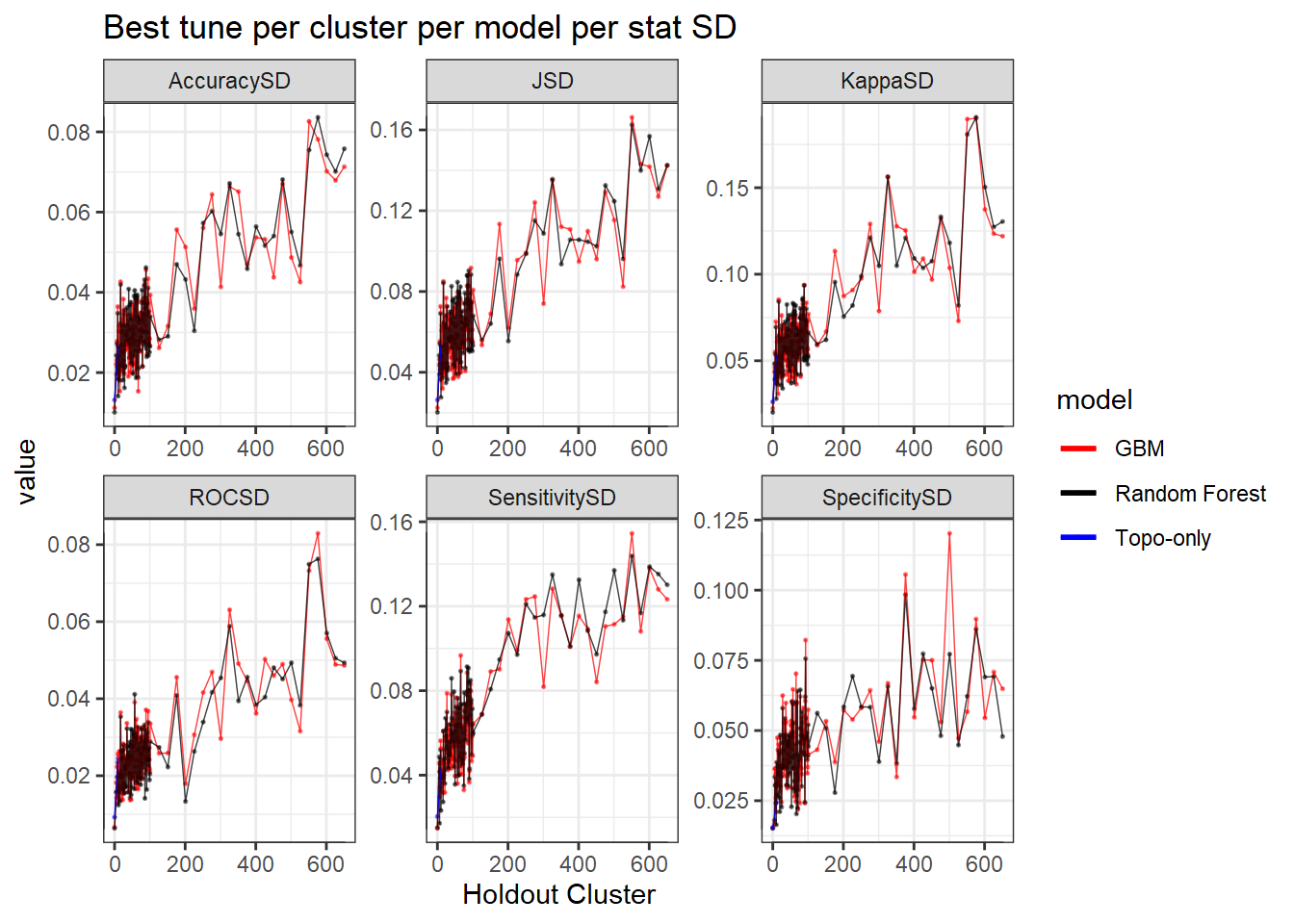
Now let’s just look at the two models side-by-side. You can see in this graph below that random forest is really overfitting with low cluster holdouts.

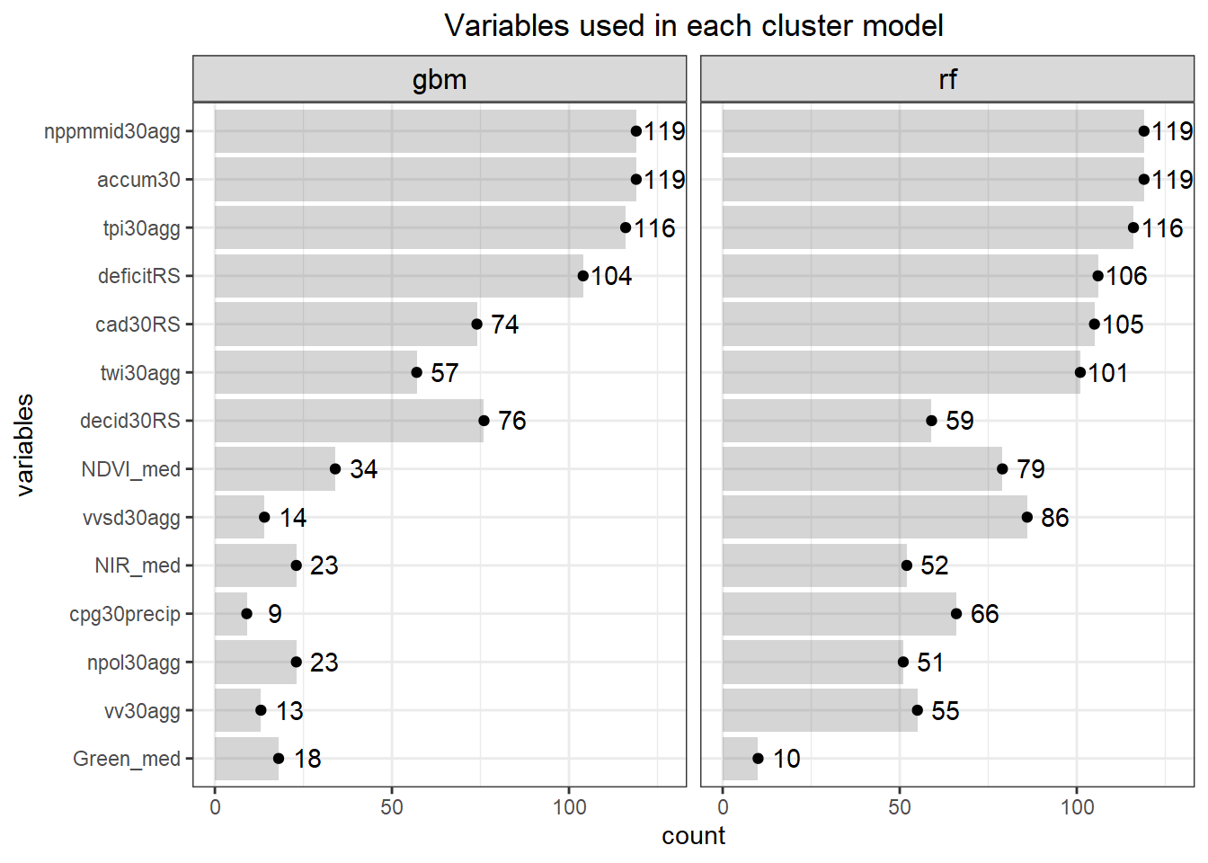
What’s really nice about doing a bunch of cluster holdouts with feature selection is we can see what variables show up the most between both models. This will give us a better idea of what variables to use instead of just selecting what ‘ffs’ selects. For example, sometimes the variable ‘Green’ gets selected in the ‘ffs’ but from the graph below both rf and gbm select ‘Green’ only a few times. So, if you just randomly choose a holdout (say 40) and get ‘Green’ now you will use this in further modelling which is going to be misleading.

If you want you can sort and play with the data below.

Here we can see that we need to make a decision about Deciduous, CAD (Cold Air Drainage) and TWI. We want to keep the variables that will provide the best results but while still keeping the model parsimonious. From the graphs above it’s evident that gbm is not as sensitive to spatial cluster when compared to rf. Both are very sensitive when using all variables and no spatial hold-out; however, when increasing the hold out size (iid becomes more appropriate) we see that rf takes some time before it stabilizes unlike gbm which is able to control for that effect early on. Not sure why this happens but it might be 1). random forest is sensitive to spatial data due to bootstrapping non-iid data which in turn overfits, 2). gbm by default does its own kind of feature selection (slow learners and no bootstrapping or mtry) which might help curb some of the spatial overfitting seen by random forest. Thus, we’ll use gbm from here on out to reduce the chance of overfitting.

Below are a couple different visualisations of how the data reacts to cluster sizes. We really want to see if there is a point at which we can ‘accept’ our model in terms of iid assumptions, i.e. has it accounted for the effects of spatial autocorrelation.

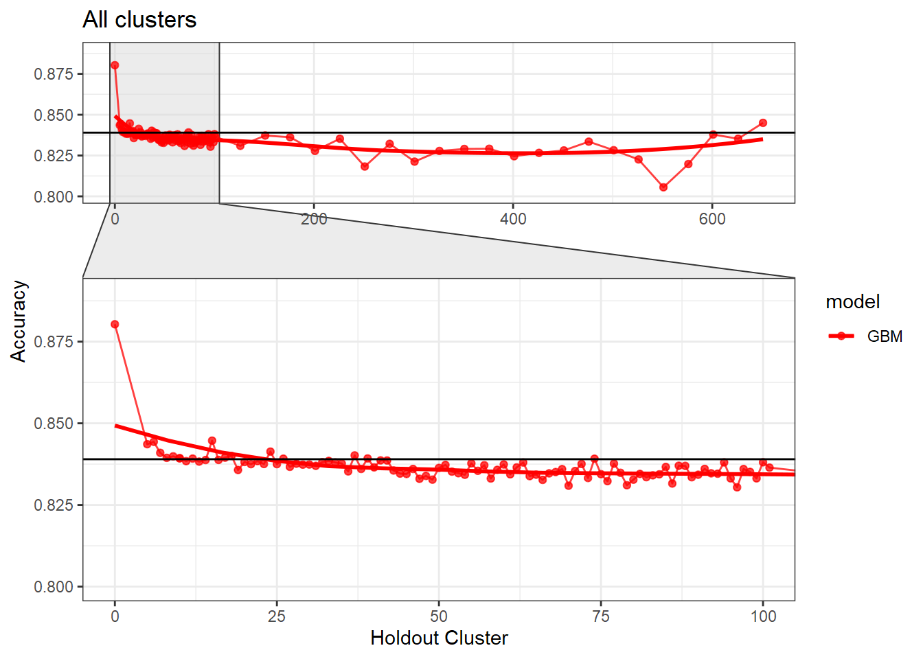
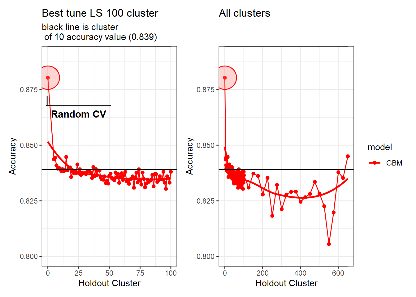
As you can see from the graphs above the black line is at the accuracy of 10 clusters. It seems that if you go beyond the clustering of 10 you slowly decrease accuracy to a point. The point at which the accuracy increases is due to unequal size of folds in the cv. This leads to folds having around 25% of the data or more within one fold! From the graphs above, it’s clear that 10 clusters is a conservative hold out value, i.e. we could pick 20, 30, 50, 100, etc and it would be relatively the same (difference between 10 and 100 is 0.001). The important part is the contrast from no holdouts (Random CV) to the 10 cluster holdout (difference between 0 and 10 is 0.041). From this I feel confident continuing with the tuning of 10 hold outs and 5 variables (accumulation, TPI, NPP, Deficit, CAD). Below you will see the range were the ‘tuned’ 10 hold out compared with the ‘ffs’ holdout.

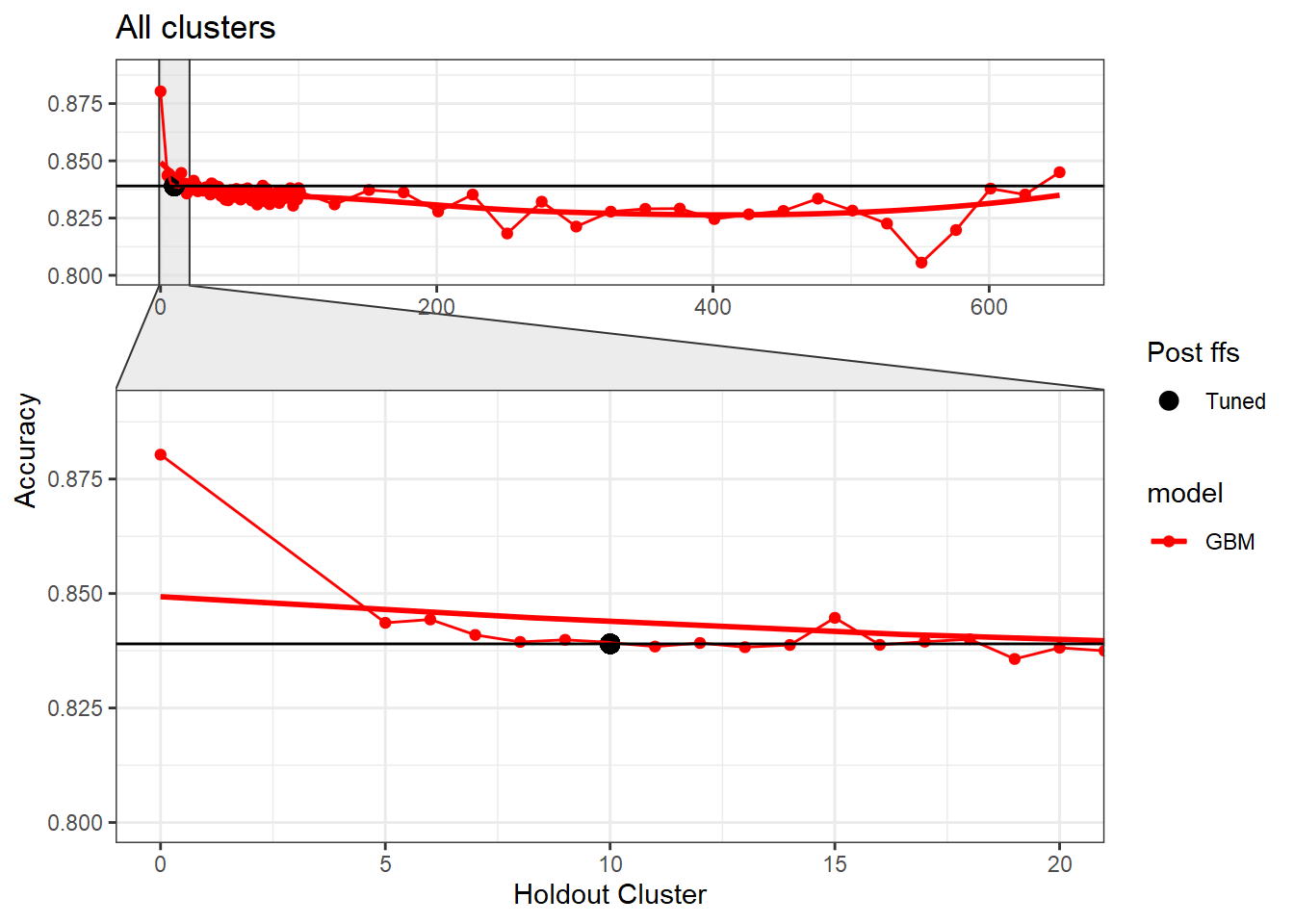
As you can see, it’s the same (0.839); however, here are the variables associated with the ffs: accum30, nppmmid30agg, deficitRS, twi30agg, tpi30agg, vv30agg, decid30RS, cad30RS, NDVI_med. Hence, we dropped from 9 to 5 and kept the accuracy the same making the model more parsimonious.